AMC 25.341  Gust and Continuous Turbulence Design Criteria (Acceptable Means of Compliance)

1.       PURPOSE. This AMC sets forth an acceptable means of compliance with the provisions of CS-25 dealing with discrete gust and continuous turbulence dynamic loads. 

2.       RELATED CERTIFICATION SPECIFICATIONS. The contents of this AMC are considered by the Agency in determining compliance with the discrete gust and continuous turbulence criteria defined in CS 25.341. Related paragraphs are:

CS 25.343             Design fuel and oil loads

CS 25.345             High lift devices

CS 25.349             Rolling conditions

CS 25.371             Gyroscopic loads

CS 25.373             Speed control devices

CS 25.391             Control surface loads

CS 25.427             Unsymmetrical loads

CS 25 445              Auxiliary aerodynamic surfaces

CS 25.571             Damage-tolerance and fatigue evaluation of structure

Reference should also be made to the following CS paragraphs: CS 25.301, CS 25.302, CS 25.303, CS 25.305, CS 25.321, CS 25.335, CS 25.1517.

3.       OVERVIEW. This AMC addresses both discrete gust and continuous turbulence (or continuous gust) requirements of CS-25. It provides some of the acceptable methods of modelling aeroplanes, aeroplane components, and configurations, and the validation of those modelling methods for the purpose of determining the response of the aeroplane to encounters with gusts.

How the various aeroplane modelling parameters are treated in the dynamic analysis can have a large influence on design load levels. The basic elements to be modelled in the analysis are the elastic, inertial, aerodynamic and control system characteristics of the complete, coupled aeroplane (Figure 1). The degree of sophistication and detail required in the modelling depends on the complexity of the aeroplane and its systems.

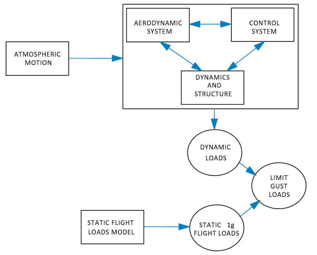
Figure 1 Basic Elements of the Gust Response Analysis

Design loads for encounters with gusts are a combination of the steady level 1-g flight loads, and the gust incremental loads including the dynamic response of the aeroplane. The steady 1-g flight loads can be realistically defined by the basic external parameters such as speed, altitude, weight and fuel load. They can be determined using static aeroelastic methods.

The gust incremental loads result from the interaction of atmospheric turbulence and aeroplane rigid body and elastic motions. They may be calculated using linear analysis methods when the aeroplane and its flight control systems are reasonably or conservatively approximated by linear analysis models.

Non-linear solution methods are necessary for aeroplane and flight control systems that are not reasonably or conservatively represented by linear analysis models. Non-linear features generally raise the level of complexity, particularly for the continuous turbulence analysis, because they often require that the solutions be carried out in the time domain. 

The modelling parameters discussed in the following paragraphs include:

—          Design conditions and associated steady, level 1-g flight conditions.

—          The discrete and continuous gust models of atmospheric turbulence.

—          Detailed representation of the aeroplane system including structural dynamics, aerodynamics, and control system modelling.

—          Solution of the equations of motion and the extraction of response loads.

—          Considerations for non-linear aeroplane systems.

—          Analytical model validation techniques.

4.       DESIGN CONDITIONS.

          a.       General. Analyses should be conducted to determine gust response loads for the aeroplane throughout its design envelope, where the design envelope is taken to include, for example, all appropriate combinations of aeroplane configuration, weight, centre of gravity, payload, fuel load, thrust, speed, and altitude.

          b.       Steady Level 1-g Flight Loads.  The total design load is made up of static and dynamic load components. In calculating the static component, the aeroplane is assumed to be in trimmed steady level flight, either as the initial condition for the discrete gust evaluation or as the mean flight condition for the continuous turbulence evaluation. Static aeroelastic effects should be taken into account if significant.

         To ensure that the maximum total load on each part of the aeroplane is obtained, the associated steady-state conditions should be chosen in such a way as to reasonably envelope the range of possible steady-state conditions that could be achieved in that flight condition. Typically, this would include consideration of effects such as speed brakes, power settings between zero thrust and the maximum for the flight condition, etc.

c.       Dynamic Response Loads.  The incremental loads from the dynamic gust solution are superimposed on the associated steady level flight 1-g loads. Load responses in both positive and negative senses should be assumed in calculating total gust response loads.  Generally the effects of speed brakes, flaps, or other drag or high lift devices, while they should be included in the steady-state condition, may be neglected in the calculation of incremental loads.

d.       Damage Tolerance Conditions. Limit gust loads, treated as ultimate, need to be developed for the structural failure conditions considered under CS 25.571(b). Generally, for redundant structures, significant changes in stiffness or geometry do not occur for the types of damage under consideration. As a result, the limit gust load values obtained for the undamaged aircraft may be used and applied to the failed structure. However, when structural failures of the types considered under CS 25.571(b) cause significant changes in stiffness or geometry, or both, these changes should be taken into account when calculating limit gust loads for the damaged structure.

5.       GUST MODEL CONSIDERATIONS.

a.       General. The gust criteria presented in CS 25.341 consist of two models of atmospheric turbulence, a discrete model and a continuous turbulence model. It is beyond the scope of this AMC to review the historical development of these models and their associated parameters. This AMC focuses on the application of those gust criteria to establish design limit loads. The discrete gust model is used to represent single discrete extreme turbulence events. The continuous turbulence model represents longer duration turbulence encounters which excite lightly damped modes. Dynamic loads for both atmospheric models must be considered in the structural design of the aeroplane.

b.       Discrete Gust Model

(1)     Atmosphere. The atmosphere is assumed to be one dimensional with the gust velocity acting normal (either vertically or laterally) to the direction of aeroplane travel. The one-dimensional assumption constrains the instantaneous vertical or lateral gust velocities to be the same at all points in planes normal to the direction of aeroplane travel. Design level discrete gusts are assumed to have 1-cosine velocity profiles. The maximum velocity for a discrete gust is calculated using a reference gust velocity, U_ref, a flight profile alleviation factor, Fg, and an expression which modifies the maximum velocity as a function of the gust gradient distance, H. These parameters are discussed further below.

(A)     Reference Gust Velocity, U_ref  - Derived effective gust velocities representing gusts occurring once in 70,000 flight hours are the basis for design gust velocities. These reference velocities are specified as a function of altitude in CS 25.341(a)(5) and are given in terms of feet per second equivalent airspeed for a gust gradient distance, H, of 107 m (350 ft).

(B)     Flight Profile Alleviation Factor, F_g - The reference gust velocity, Uref , is a measure of turbulence intensity as a function of altitude. In defining the value of Uref at each altitude, it is assumed that the aircraft is flown 100% of the time at that altitude. The factor F_g is then applied to account for the expected service experience in terms of the probability of the aeroplane flying at any given altitude within its certification altitude range. Fg is a minimum value at sea level, linearly increasing to 1.0 at the certified maximum altitude. The expression for Fg is given in CS 25.341(a)(6).

(C)     Gust Gradient Distance, H - The gust gradient distance is that distance over which the gust velocity increases to a maximum value. Its value is specified as ranging from 9.1 to 107 m (30 to 350 ft). (It should be noted that if 12.5 times the mean geometric chord of the aeroplane’s wing exceeds 350 ft, consideration should be given to covering increased maximum gust gradient distances.)

(D)     Design Gust Velocity, U_ds - Maximum velocities for design gusts are proportional to the sixth root of the gust gradient distance, H. The maximum gust velocity for a given gust is then defined as:

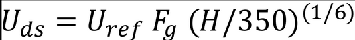
The maximum design gust velocity envelope, Uds, and example design gust velocity profiles are illustrated in Figure 2.

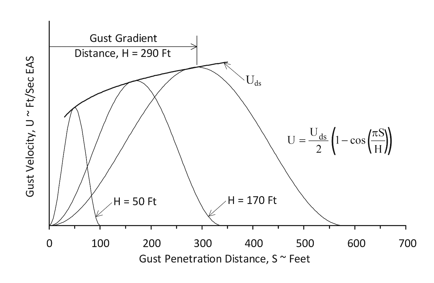
Figure-2  Typical (1-cosine) Design Gust Velocity Profiles

(2)     Discrete Gust Response. The solution for discrete gust response time histories can be achieved by a number of techniques. These include the explicit integration of the aeroplane equations of motion in the time domain, and frequency domain solutions utilising Fourier transform techniques. These are discussed further in Paragraph 7.0 of this AMC.

Maximum incremental loads, P_Ii, are identified by the peak values selected from time histories arising from a series of separate, 1-cosine shaped gusts having gradient distances ranging from 9.1 to 107 m (30 to 350 ft). Input gust profiles should cover this gradient distance range in sufficiently small increments to determine peak loads and responses. Historically 10 to 20 gradient distances have been found to be acceptable. Both positive and negative gust velocities should be assumed in calculating total gust response loads. It should be noted that in some cases, the peak incremental loads can occur well after the prescribed gust velocity has returned to zero.  In such cases, the gust response calculation should be run for sufficient additional time to ensure that the critical incremental loads are achieved.

The design limit load, P_Li , corresponding to the maximum incremental load, P_Ii for a given load quantity is then defined as:

Where P_(1-g)i is the 1-g steady load for the load quantity under consideration. The set of time correlated design loads, P_Lj , corresponding to the peak value of the load quantity, P_Li, are calculated for the same instant in time using the expression:

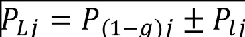
Note that in the case of a non-linear aircraft, maximum positive incremental loads may differ from maximum negative incremental loads.

         When calculating stresses which depend on a combination of external loads it may be necessary to consider time correlated load sets at time instants other than those which result in peaks for individual external load quantities.

(3)     Round-The-Clock Gust. When the effect of combined vertical and lateral gusts on aeroplane components is significant, then round-the-clock analysis should be conducted on these components and supporting structures. The vertical and lateral components of the gust are assumed to have the same gust gradient distance, H and to start at the same time. Components that should be considered include horizontal tail surfaces having appreciable dihedral or anhedral (i.e., greater than 10º), or components supported by other lifting surfaces, for example T-tails, outboard fins and winglets. Whilst the round-the-clock load assessment may be limited to just the components under consideration, the loads themselves should be calculated from a whole aeroplane dynamic analysis.

The round-the-clock gust model assumes that discrete gusts may act at any angle normal to the flight path of the aeroplane. Lateral and vertical gust components are correlated since the round-the-clock gust is a single discrete event. For a linear aeroplane system, the loads due to a gust applied from a direction intermediate to the vertical and lateral directions - the round-the-clock gust loads - can be obtained using a linear combination of the load time histories induced from pure vertical and pure lateral gusts. The resultant incremental design value for a particular load of interest is obtained by determining the round-the-clock gust angle and gust length giving the largest (tuned) response value for that load. The design limit load is then obtained using the expression for P_L given above in paragraph 5(b)(2).

(4)     Supplementary Gust Conditions for Wing Mounted Engines.

(A)     Atmosphere - For aircraft equipped with wing mounted engines, CS 25.341(c) requires that engine mounts, pylons and wing supporting structure be designed to meet a round-the-clock discrete gust requirement and a multi-axis discrete gust requirement.

The model of the atmosphere and the method for calculating response loads for the round-the-clock gust requirement is the same as that described in Paragraph 5(b)(3) of this AMC.

For the multi-axis gust requirement, the model of the atmosphere consists of two independent discrete gust components, one vertical and one lateral, having amplitudes such that the overall probability of the combined gust pair is the same as that of a single discrete gust as defined by CS 25.341(a) as described in Paragraph 5(b)(1) of this AMC. To achieve this equal-probability condition, in addition to the reductions in gust amplitudes that would be applicable if the input were a multi-axis Gaussian process, a further factor of 0.85 is incorporated into the gust amplitudes to account for non-Gaussian properties of severe discrete gusts. This factor was derived from severe gust data obtained by a research aircraft specially instrumented to measure vertical and lateral gust components. This information is contained in Stirling Dynamics Laboratories Report No SDL –571-TR-2 dated May 1999.

(B)     Multi-Axis Gust Response - For a particular aircraft flight condition, the calculation of a specific response load requires that the amplitudes, and the time phasing, of the two gust components be chosen, subject to the condition on overall probability specified in (A) above, such that the resulting combined load is maximised. For loads calculated using a linear aircraft model, the response load may be based upon the separately tuned vertical and lateral discrete gust responses for that load, each calculated as described in Paragraph 5(b)(2) of this AMC. In general, the vertical and lateral tuned gust lengths and the times to maximum response (measured from the onset of each gust) will not be the same.

Denote the independently tuned vertical and lateral incremental responses for a particular aircraft flight condition and load quantity i by L_Vi and L_Li, respectively. The associated multi-axis gust input is obtained by multiplying the amplitudes of the independently-tuned vertical and lateral discrete gusts, obtained as described in the previous paragraph, by 0.85*L_Vi/√ (L_Vi²+L_Li²) and 0.85*L_Li/√ (L_Vi²+L_Li²) respectively. The time-phasing of the two scaled gust components is such that their associated peak loads occur at the same instant.

The combined incremental response load is given by:

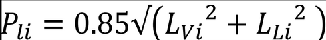
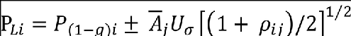
and the design limit load, P_Li, corresponding to the maximum incremental load, P_Ii, for the given load quantity is then given by:

where P_(1-g)i is the 1-g steady load for the load quantity under consideration.

The incremental, time correlated loads corresponding to the specific flight condition under consideration are obtained from the independently-tuned vertical and lateral gust inputs for load quantity i.  The vertical and lateral gust amplitudes are factored by 0.85*L_Vi/√ (L_Vi²+L_Li²) and 0.85*L_Li/√(L_Vi²+L_Li²) respectively. Loads L_Vj and L_Lj resulting from these reduced vertical and lateral gust inputs, at the time when the amplitude of load quantity i is at a maximum value, are added to yield the multi-axis incremental time-correlated value P_Ij for load quantity j.

The set of time correlated design loads, P_Lj , corresponding to the peak value of the load quantity, P_Li, are obtained using the expression:

Note that with significant non-linearities, maximum positive incremental loads may differ from maximum negative incremental loads.

c.       Continuous Turbulence Model.

(1)     Atmosphere. The atmosphere for the determination of continuous gust responses is assumed to be one dimensional with the gust velocity acting normal (either vertically or laterally) to the direction of aeroplane travel. The one-dimensional assumption constrains the instantaneous vertical or lateral gust velocities to be the same at all points in planes normal to the direction of aeroplane travel.

The random atmosphere is assumed to have a Gaussian distribution of gust velocity intensities and a Von Kármán power spectral density with a scale of turbulence, L, equal to 2500 feet. The expression for the Von Kármán spectrum for unit, root-mean-square (RMS) gust intensity, Φ_I(Ω), is given below. In this expression Ω = ω/V, where ω is the circular frequency in radians per second, and V is the aeroplane velocity in feet per second true airspeed.

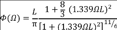
The Von Kármán power spectrum for unit RMS gust intensity is illustrated in Figure 3.

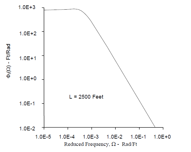
Figure-3  The Von Kármán Power Spectral Density Function, Φ_I(Ω)

         The design gust velocity, Uσ, applied in the analysis is given by the product of the reference gust velocity, Uσref , and the profile alleviation factor, Fg, as follows:

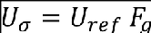
where values for Uσref , are specified in CS 25.341(b)(3) in meters per second (feet per second) true airspeed and Fg is defined in CS 25.341(a)(6). The value of Fg is based on aeroplane design parameters and is a minimum value at sea level, linearly increasing to 1.0 at the certified maximum design altitude. It is identical to that used in the discrete gust analysis.

As for the discrete gust analysis, the reference continuous turbulence gust intensity, Uσref, defines the design value of the associated gust field at each altitude. In defining the value of Uσref at each altitude, it is assumed that the aeroplane is flown 100% of the time at that altitude. The factor Fg is then applied to account for the probability of the aeroplane flying at any given altitude during its service lifetime.

It should be noted that the reference gust velocity is comprised of two components, a root-mean-square (RMS) gust intensity and a peak to RMS ratio. The separation of these components is not defined and is not required for the linear aeroplane analysis. Guidance is provided in Paragraph 8.d. of this AMC for generating a RMS gust intensity for a non-linear simulation.

(2)     Continuous Turbulence Response. For linear aeroplane systems, the solution for the response to continuous turbulence may be performed entirely in the frequency domain, using the RMS response. is defined in CS 25.341(b)(2) and is repeated here in modified notation for load quantity i, where:

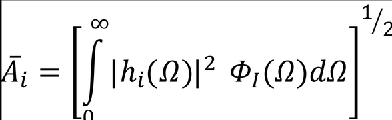
or

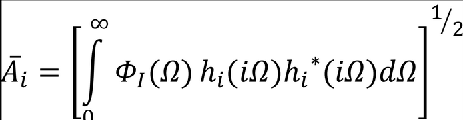
In the above expression Φ_I(Ω) is the input Von Kármán power spectrum of the turbulence and is defined in Paragraph 5.c.(1) of this AMC, h_i(iΩ) is the transfer function relating the output load quantity, i, to a unit, harmonically oscillating, one-dimensional gust field, and the asterisk superscript denotes the complex conjugate. When evaluating Ā_i, the integration should be continued until a converged value is achieved since, realistically, the integration to infinity may be impractical. The design limit load, P_Li, is then defined as:

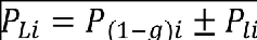
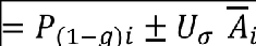
where U_σ is defined in Paragraph 5.c.(1) of this AMC, and P_(1-g)i is the 1-g steady state value for the load quantity, i, under consideration. As indicated by the formula, both positive and negative load responses should be considered when calculating limit loads.

Correlated (or equiprobable) loads can be developed using cross-correlation coefficients, ρ_ij, computed as follows:

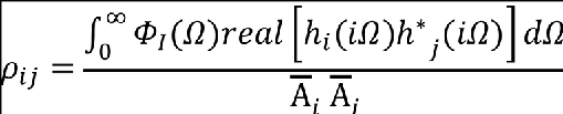
where, ‘real[...]’ denotes the real part of the complex function contained within the brackets. In this equation, the lowercase subscripts, i and j, denote the responses being correlated. A set of design loads, P_Lj, correlated to the design limit load P_Li, are then calculated as follows:

The correlated load sets calculated in the foregoing manner provide balanced load distributions corresponding to the maximum value of the response for each external load quantity, i, calculated.

When calculating stresses, the foregoing load distributions may not yield critical design values because critical stress values may depend on a combination of external loads. In these cases, a more general application of the correlation coefficient method is required. For example, when the value of stress depends on two externally applied loads, such as torsion and shear, the equiprobable relationship between the two parameters forms an ellipse as illustrated in Figure 4.

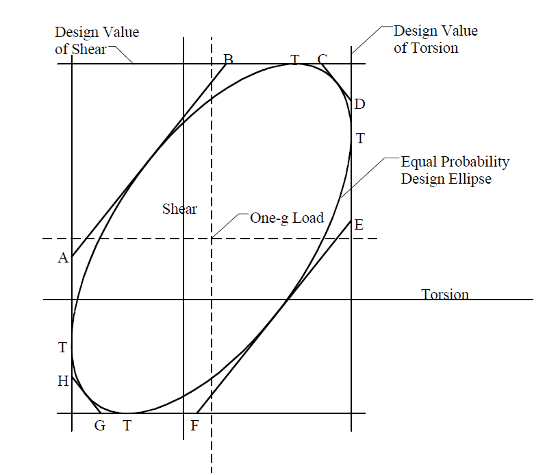
Figure-4  Equal Probability Design Ellipse

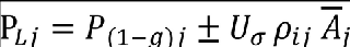
In this figure, the points of tangency, T, correspond to the expressions for correlated load pairs given by the foregoing expressions. A practical additional set of equiprobable load pairs that should be considered to establish critical design stresses are given by the points of tangency to the ellipse by lines AB, CD, EF and GH. These additional load pairs are given by the following expressions (where i = torsion and j = shear):

For tangents to lines AB and EF

and

For tangents to lines CD and GH

and

All correlated or equiprobable loads developed using correlation coefficients will provide balanced load distributions.

A more comprehensive approach for calculating critical design stresses that depend on a combination of external load quantities is to evaluate directly the transfer function for the stress quantity of interest from which can be calculated the gust response function, the value for RMS response, Ā, and the design stress values P(1-g) ± U_σ Ā.

6.       AEROPLANE MODELLING CONSIDERATIONS

a.       General. The procedures presented in this paragraph generally apply for aeroplanes having aerodynamic and structural properties and flight control systems that may be reasonably or conservatively approximated using linear analysis methods for calculating limit load. Additional guidance material is presented in Paragraph 8 of this AMC for aeroplanes having properties and/or systems not reasonably or conservatively approximated by linear analysis methods.

b.       Structural Dynamic Model. The model should include both rigid body and flexible aeroplane degrees of freedom. If a modal approach is used, the structural dynamic model should include a sufficient number of flexible aeroplane modes to ensure both convergence of the modal superposition procedure and that responses from high frequency excitations are properly represented.

Most forms of structural modelling can be classified into two main categories: (1) the so-called “stick model” characterised by beams with lumped masses distributed along their lengths, and (2) finite element models in which all major structural components (frames, ribs, stringers, skins) are represented with mass properties defined at grid points. Regardless of the approach taken for the structural modelling, a minimum acceptable level of sophistication, consistent with configuration complexity, is necessary to represent satisfactorily the critical modes of deformation of the primary structure and control surfaces. Results from the models should be compared to test data as outlined in Paragraph 9.b. of this AMC in order to validate the accuracy of the model.

c.       Structural Damping.  Structural dynamic models may include damping properties in addition to representations of mass and stiffness distributions. In the absence of better information it will normally be acceptable to assume 0.03 (i.e. 1.5% equivalent critical viscous damping) for all flexible modes. Structural damping may be increased over the 0.03 value to be consistent with the high structural response levels caused by extreme gust intensity, provided justification is given.

d.       Gust and Motion Response Aerodynamic Modelling. Aerodynamic forces included in the analysis are produced by both the gust velocity directly, and by the aeroplane response.

Aerodynamic modelling for dynamic gust response analyses requires the use of unsteady two-dimensional or three-dimensional panel theory methods for incompressible or compressible flow. The choice of the appropriate technique depends on the complexity of the aerodynamic configuration, the dynamic motion of the surfaces under investigation and the flight speed envelope of the aeroplane. Generally, three-dimensional panel methods achieve better modelling of the aerodynamic interference between lifting surfaces. The model should have a sufficient number of aerodynamic degrees of freedom to properly represent the steady and unsteady aerodynamic distributions under consideration.

The build-up of unsteady aerodynamic forces should be represented. In two-dimensional unsteady analysis this may be achieved in either the frequency domain or the time domain through the application of oscillatory or indicial lift functions, respectively. Where three-dimensional panel aerodynamic theories are to be applied in the time domain (e.g. for non-linear gust solutions), an approach such as the ‘rational function approximation’ method may be employed to transform frequency domain aerodynamics into the time domain.

Oscillatory lift functions due to gust velocity or aeroplane response depend on the reduced frequency parameter, k. The maximum reduced frequency used in the generation of the unsteady aerodynamics should include the highest frequency of gust excitation and the highest structural frequency under consideration. Time lags representing the effect of the gradual penetration of the gust field by the aeroplane should also be accounted for in the build-up of lift due to gust velocity.

The aerodynamic modelling should be supported by tests or previous experience as indicated in Paragraph 9.d. of this AMC. Primary lifting and control surface distributed aerodynamic data are commonly adjusted by weighting factors in the dynamic gust response analyses. The weighting factors for steady flow (k = 0) may be obtained by comparing wind tunnel test results with theoretical data. The correction of the aerodynamic forces should also ensure that the rigid body motion of the aeroplane is accurately represented in order to provide satisfactory short period and Dutch roll frequencies and damping ratios. Corrections to primary surface aerodynamic loading due to control surface deflection should be considered.  Special attention should also be given to control surface hinge moments and to fuselage and nacelle aerodynamics because viscous and other effects may require more extensive adjustments to the theoretical coefficients. Aerodynamic gust forces should reflect weighting factor adjustments performed on the steady or unsteady motion response aerodynamics.

e.       Gyroscopic Loads. As specified in CS 25.371, the structure supporting the engines and the auxiliary power units should be designed for the gyroscopic loads induced by both discrete gusts and continuous turbulence. The gyroscopic loads for turbopropellers and turbofans may be calculated as an integral part of the solution process by including the gyroscopic terms in the equations of motion or the gyroscopic loads can be superimposed after the solution of the equations of motion. Propeller and fan gyroscopic coupling forces (due to rotational direction) between symmetric and antisymmetric modes need not be taken into account if the coupling forces are shown to be negligible.

The gyroscopic loads used in this analysis should be determined with the engine or auxiliary power units at maximum continuous rpm. The mass polar moment of inertia used in calculating gyroscopic inertia terms should include the mass polar moments of inertia of all significant rotating parts taking into account their respective rotational gearing ratios and directions of rotation.

f.       Control Systems. Gust analyses of the basic configuration should include simulation of any control system for which interaction may exist with the rigid body response, structural dynamic response or external loads. If possible, these control systems should be uncoupled such that the systems which affect “symmetric flight” are included in the vertical gust analysis and those which affect “antisymmetric flight” are included in the lateral gust analysis.

The control systems considered should include all relevant modes of operation. Failure conditions should also be analysed for any control system which influences the design loads in accordance with CS 25.302 and Appendix K.

The control systems included in the gust analysis may be assumed to be linear if the impact of the non-linearity is negligible, or if it can be shown by analysis on a similar aeroplane/control system that a linear control law representation is conservative. If the control system is significantly non-linear, and a conservative linear approximation to the control system cannot be developed, then the effect of the control system on the aeroplane responses should be evaluated in accordance with Paragraph 8. of this AMC.

g.       Stability. Solutions of the equations of motion for either discrete gusts or continuous turbulence require the dynamic model be stable. This applies for all modes, except possibly for very low frequency modes which do not affect load responses, such as the phugoid mode. (Note that the short period and Dutch roll modes do affect load responses). A stability check should be performed for the dynamic model using conventional stability criteria appropriate for the linear or non-linear system in question, and adjustments should be made to the dynamic model, as required, to achieve appropriate frequency and damping characteristics.

         If control system models are to be included in the gust analysis it is advisable to check that the following characteristics are acceptable and are representative of the aeroplane:

—         static margin of the unaugmented aeroplane

—         dynamic stability of the unaugmented aeroplane

—         the static aeroelastic effectiveness of all control surfaces utilised by any feed-back control system

—         gain and phase margins of any feedback control system coupled with the aeroplane rigid body and flexible modes

—         the aeroelastic flutter and divergence margins of the unaugmented aeroplane, and also for any feedback control system coupled with the aeroplane.

7.       DYNAMIC LOADS

a.       General. This paragraph describes methods for formulating and solving the aeroplane equations of motion and extracting dynamic loads from the aeroplane response. The aeroplane equations of motion are solved in either physical or modal co-ordinates and include all terms important in the loads calculation including stiffness, damping, mass, and aerodynamic forces due to both aeroplane motions and gust excitation. Generally the aircraft equations are solved in modal co-ordinates. For the purposes of describing the solution of these equations in the remainder of this AMC, modal co-ordinates will be assumed. A sufficient number of modal co-ordinates should be included to ensure that the loads extracted provide converged values.

b.       Solution of the Equations of Motion. Solution of the equations of motion can be achieved through a number of techniques. For the continuous turbulence analysis, the equations of motion are generally solved in the frequency domain. Transfer functions which relate the output response quantity to an input harmonically oscillating gust field are generated and these transfer functions are used (in Paragraph 5.c. of this AMC) to generate the RMS value of the output response quantity.

There are two primary approaches used to generate the output time histories for the discrete gust analysis; (1) by explicit integration of the aeroplane equations of motion in the time domain, and (2) by frequency domain solutions which can utilise Fourier transform techniques.

c.       Extraction of Loads and Responses.  The output quantities that may be extracted from a gust response analysis include displacements, velocities and accelerations at structural locations; load quantities such as shears, bending moments and torques on structural components; and stresses and shear flows in structural components. The calculation of the physical responses is given by a modal superposition of the displacements, velocities and accelerations of the rigid and elastic modes of vibration of the aeroplane structure. The number of modes carried in the summation should be sufficient to ensure converged results.

A variety of methods may be used to obtain physical structural loads from a solution of the modal equations of motion governing gust response. These include the Mode Displacement method, the Mode Acceleration method, and the Force Summation method. All three methods are capable of providing a balanced set of aeroplane loads. If an infinite number of modes can be considered in the analysis, the three will lead to essentially identical results.

The Mode Displacement method is the simplest. In this method, total dynamic loads are calculated from the structural deformations produced by the gust using modal superposition. Specifically, the contribution of a given mode is equal to the product of the load associated with the normalised deformed shape of that mode and the value of the displacement response given by the associated modal co-ordinate. For converged results, the Mode Displacement method may need a significantly larger number of modal co-ordinates than the other two methods. 

In the Mode Acceleration method, the dynamic load response is composed of a static part and a dynamic part. The static part is determined by conventional static analysis (including rigid body “inertia relief”), with the externally applied gust loads treated as static loads. The dynamic part is computed by the superposition of appropriate modal quantities, and is a function of the number of modes carried in the solution. The quantities to be superimposed involve both motion response forces and acceleration responses (thus giving this method its name). Since the static part is determined completely and independently of the number of normal modes carried, adequate accuracy may be achieved with fewer modes than would be needed in the Mode Displacement method.

The Force Summation method is the most laborious and the most intuitive. In this method, physical displacements, velocities and accelerations are first computed by superposition of the modal responses. These are then used to determine the physical inertia forces and other motion dependent forces. Finally, these forces are added to the externally applied forces to give the total dynamic loads acting on the structure.

If balanced aeroplane load distributions are needed from the discrete gust analysis, they may be determined using time correlated solution results.  Similarly, as explained in Paragraph 5.c of this AMC, if balanced aeroplane load distributions are needed from the continuous turbulence analysis, they may be determined from equiprobable solution results obtained using cross-correlation coefficients.

8.       NONLINEAR CONSIDERATIONS

a.       General. Any structural, aerodynamic or automatic control system characteristic which may cause aeroplane response to discrete gusts or continuous turbulence to become non-linear with respect to intensity or shape should be represented realistically or conservatively in the calculation of loads. While many minor non-linearities are amenable to a conservative linear solution, the effect of major non-linearities cannot usually be quantified without explicit calculation.

The effect of non-linearities should be investigated above limit conditions to assure that the system presents no anomaly compared to behaviour below limit conditions, in accordance with Appendix K, K25.2(b)(2).

b.       Structural and Aerodynamic Non-linearity. A linear elastic structural model, and a linear (unstalled) aerodynamic model are normally recommended as conservative and acceptable for the unaugmented aeroplane elements of a loads calculation. Aerodynamic models may be refined to take account of minor non-linear variation of aerodynamic distributions, due to local separation etc., through simple linear piecewise solution. Local or complete stall of a lifting surface would constitute a major non-linearity and should not be represented without account being taken of the influence of rate of change of incidence, i.e., the so-called ‘dynamic stall’ in which the range of linear incremental aerodynamics may extend significantly beyond the static stall incidence.

c.       Automatic Control System Non-linearity. Automatic flight control systems, autopilots, stability control systems and load alleviation systems often constitute the primary source of non-linear response. For example,

—         non-proportional feedback gains

—         rate and amplitude limiters

—         changes in the control laws, or control law switching

—         hysteresis

—         use of one-sided aerodynamic controls such as spoilers

—         hinge moment performance and saturation of aerodynamic control actuators

The resulting influences on response will be aeroplane design dependent, and the manner in which they are to be considered will normally have to be assessed for each design.

Minor influences such as occasional clipping of response due to rate or amplitude limitations, where it is symmetric about the stabilised 1-g condition, can often be represented through quasi-linear modelling techniques such as describing functions or use of a linear equivalent gain.

Major, and unsymmetrical influences such as application of spoilers for load alleviation, normally require explicit simulation, and therefore adoption of an appropriate solution based in the time domain.

The influence of non-linearities on one load quantity often runs contrary to the influence on other load quantities. For example, an aileron used for load alleviation may simultaneously relieve wing bending moment whilst increasing wing torsion. Since it may not be possible to represent such features conservatively with a single aeroplane model, it may be conservatively acceptable to consider loads computed for two (possibly linear) representations which bound the realistic condition. Another example of this approach would be separate representation of continuous turbulence response for the two control law states to cover a situation where the aeroplane may occasionally switch from one state to another.

d.       Non-linear Solution Methodology.  Where explicit simulation of non-linearities is required, the loads response may be calculated through time domain integration of the equations of motion.

For the tuned discrete gust conditions of CS 25.341(a), limit loads should be identified by peak values in the non-linear time domain simulation response of the aeroplane model excited by the discrete gust model described in Paragraph 5.b. of this AMC.

For time domain solution of the continuous turbulence conditions of CS 25.341(b), a variety of approaches may be taken for the specification of the turbulence input time history and the mechanism for identifying limit loads from the resulting responses.

It will normally be necessary to justify that the selected approach provides an equivalent level of safety as a conventional linear analysis and is appropriate to handle the types of non-linearity on the aircraft. This should include verification that the approach provides adequate statistical significance in the loads results.

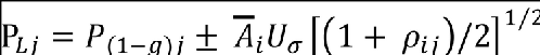
A methodology based upon stochastic simulation has been found to be acceptable for load alleviation and flight control system non-linearities. In this simulation, the input is a long, Gaussian, pseudo-random turbulence stream conforming to a Von Kármán spectrum with a root-mean-square (RMS) amplitude of 0.4 times U_σ (defined in Paragraph 5.c (1) of this AMC). The value of limit load is that load with the same probability of exceedance as Ā U_σ of the same load quantity in a linear model. This is illustrated graphically in Figure 5. When using an analysis of this type, exceedance curves should be constructed using incremental load values up to, or just beyond the limit load value.

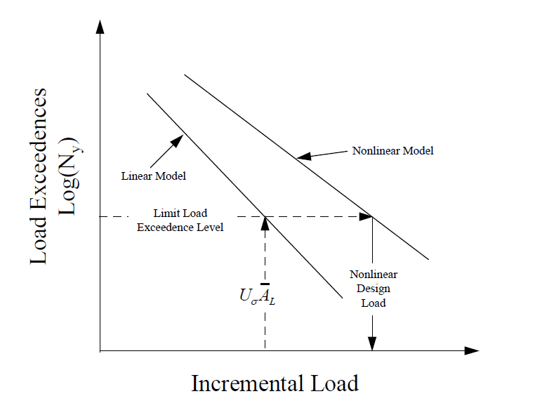
Figure-5  Establishing Limit Load for a Non-linear Aeroplane

The non-linear simulation may also be performed in the frequency domain if the frequency domain method is shown to produce conservative results. Frequency domain methods include, but are not limited to, Matched Filter Theory and Equivalent Linearisation.

9.       ANALYTICAL MODEL VALIDATION

a.       General. The intent of analytical model validation is to establish that the analytical model is adequate for the prediction of gust response loads. The following paragraphs discuss acceptable but not the only methods of validating the analytical model. In general, it is not intended that specific testing be required to validate the dynamic gust loads model.

b.       Structural Dynamic Model Validation. The methods and test data used to validate the flutter analysis models presented in AMC 25.629 should also be applied to validate the gust analysis models. These procedures are addressed in AMC 25.629.

c.       Damping Model Validation. In the absence of better information it will normally be acceptable to assume 0.03 (i.e. 1.5% equivalent critical viscous damping) for all flexible modes. Structural damping may be increased over the 0.03 value to be consistent with the high structural response levels caused by extreme gust intensity, provided justification is given.

d.       Aerodynamic Model Validation. Aerodynamic modelling parameters fall into two categories:

(i)      steady or quasi-steady aerodynamics governing static aeroelastic and flight dynamic airload distributions

(ii)     unsteady aerodynamics which interact with the flexible modes of the aeroplane.

Flight stability aerodynamic distributions and derivatives may be validated by wind tunnel tests, detailed aerodynamic modelling methods (such as CFD) or flight test data. If detailed analysis or testing reveals that flight dynamic characteristics of the aeroplane differ significantly from those to which the gust response model have been matched, then the implications on gust loads should be investigated.

The analytical and experimental methods presented in AMC 25.629 for flutter analyses provide acceptable means for establishing reliable unsteady aerodynamic characteristics both for motion response and gust excitation aerodynamic force distributions. The aeroelastic implications on aeroplane flight dynamic stability should also be assessed.

e.       Control System Validation. If the aeroplane mathematical model used for gust analysis contains a representation of any feedback control system, then this segment of the model should be validated. The level of validation that should be performed depends on the complexity of the system and the particular aeroplane response parameter being controlled. Systems which control elastic modes of the aeroplane may require more validation than those which control the aeroplane rigid body response. Validation of elements of the control system (sensors, actuators, anti-aliasing filters, control laws, etc.) which have a minimal effect on the output load and response quantities under consideration can be neglected.

It will normally be more convenient to substantiate elements of the control system independently, i.e. open loop, before undertaking the validation of the closed loop system.

(1)     System Rig or Aeroplane Ground Testing. Response of the system to artificial stimuli can be measured to verify the following:

—         The transfer functions of the sensors and any pre-control system anti-aliasing or other filtering.

—         The sampling delays of acquiring data into the control system.

—         The behaviour of the control law itself.

—         Any control system output delay and filter transfer function.

—         The transfer functions of the actuators, and any features of actuation system performance characteristics that may influence the actuator response to the maximum demands that might arise in turbulence; e.g. maximum rate of deployment, actuator hinge moment capability, etc.

If this testing is performed, it is recommended that following any adaptation of the model to reflect this information, the complete feedback path be validated (open loop) against measurements taken from the rig or ground tests.

(2)     Flight Testing. The functionality and performance of any feedback control system can also be validated by direct comparison of the analytical model and measurement for input stimuli. If this testing is performed, input stimuli should be selected such that they exercise the features of the control system and the interaction with the aeroplane that are significant in the use of the mathematical model for gust load analysis. These might include:

—         Aeroplane response to pitching and yawing manoeuvre demands.

—         Control system and aeroplane response to sudden artificially introduced demands such as pulses and steps.

—         Gain and phase margins determined using data acquired within the flutter test program. These gain and phase margins can be generated by passing known signals through the open loop system during flight test.

[Amdt No: 25/1]

[Amdt No: 25/23]