Appendix 2 to ETSO-C117b – Wind Field Models and Data

This Appendix contains data that defines the wind field models to be used in conducting the tests specified in paragraph 4(d)(10) of this ETSO. This material was developed by the National Aeronautics And Space Administration (NASA), reference NASA Technical Memorandum 100632 [ref. 1].

The downburst model parameters below provide the variables to be used to obtain the representative test conditions: (1) and (2)

(1) From analytic microburst model documented in NASA TM-100632. These parameters are based on data from Proctor’s Terminal Area Simulation System (TASS) model.

(2) For the takeoff case, the downburst centre is positioned at the point the aeroplane lifts off the runway for all test cases.

(3) For the approach/landing case, the downburst centre is positioned as stated. The test is begun with the aeroplane at an initial altitude of 1 500 feet on a 3° glideslope (touchdown point approximately 29 000 feet away). The distance from the starting point indicates where the centre of the downburst shaft is located relative to the starting point. The number in parentheses next to it indicates the relative distance of the microburst centre from the touchdown point (not the end of the runway). A negative number indicates that the microburst centre is located before the touchdown point, positive indicates it is past the touchdown point.

SUMMARY

A simple downburst model has been developed for use in batch and real-time piloted simulation studies of guidance strategies for terminal area transport aeroplane operations in wind shear conditions. The model represents an axisymmetric stagnation point flow, based on velocity profiles from the Terminal Area Simulation System (TASS) model developed by Proctor [ref. 3,4] and satisfies the mass continuity equation in cylindrical coordinates. Altitude dependence, including boundary layer effects near the ground, closely matches real-world measurements, as do the increase, peak, and decay of outflow and downflow with increasing distance from the downburst centre. Equations for horizontal and vertical winds were derived, and found to be infinitely differentiable, with no singular points existent in the flow field. In addition, a simple relationship exists among the ratio of maximum horizontal to vertical velocities, the downdraft radius, depth of outflow, and altitude of maximum outflow. In use, a microburst can be modelled by specifying four characteristic parameters. Velocity components in the x, y, and z directions, and the corresponding nine partial derivatives are obtained easily from the velocity equations.

INTRODUCTION

Terminal area operation of transport aircraft in a wind shear environment has been recognised as a serious problem. Studies of aeroplanes trajectories through downbursts show that specific guidance strategies are needed for aeroplanes to survive inadvertent downburst encounters. In order for guidance strategies to perform in simulations as in actual encounters, a realistic set of conditions must be present during development of the strategies. Thus, aeroplane and wind models that closely simulate real-world conditions are essential in obtaining useful information from the studies.

Wind models for use on personal computers, or for simulators with limited memory space availability, have been difficult to obtain because variability of downburst characteristics makes analytical models unrealistic, and large memory requirements make the use of numerical models impossible on any except very large capacity computers.

Bray [ref. 2] developed a method for analytic modelling of wind shear conditions in flight simulators, and applied his method in modelling a multiple downburst scenario from Joint Airport Weather Studies (JAWS) data. However, the altitude dependence of his model is not consistent with observed data and, although flexibility in sizing the downbursts is built into the model, it does not maintain the physical relationships which are seen in real-world data among the sizing parameters. In particular, boundary layer effects should cause the radial velocity to decay vertically to zero at the ground, as does the vertical velocity.

In a study conducted at NASA Langley Research Center, three different guidance strategies for a Boeing 737-100 aeroplane encountering a microburst on take-off were developed [ref. 3-4]. These strategies were first developed using a personal computer, and then implemented in a pilot-in-the-loop simulation using a very simple wind model in both efforts. The wind velocities used are depicted in Figure 1. This model consisted of a constant outflow outside of the downburst radius and a constant slope headwind to tailwind shear across the diameter of the downburst.

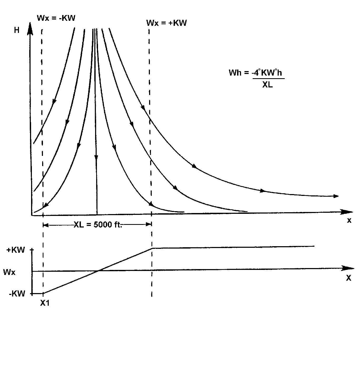
Figure 1 — Wind Model Used in Guidance Studies

It was recognised that a more realistic wind model could significantly alter the outcome of the trajectory. For the subsequent part of this study, which involves altering the aeroplane model to simulate approach to landing and escape manoeuvres and additional take-off cases, a more realistic wind model was preferred. The simple analytical model outlined in this report was developed for this purpose.

SYMBOLS

DEVELOPMENT OF VELOCITY EQUATIONS

Beginning with the full set of Euler and mass continuity equations, some simplifying assumptions about the downburst flow conditions were made. Effects of viscosity were parameterised explicitly, and the flow was assumed to be invariant with time. The downburst is axisymmetric in cylindrical coordinates, and characterized by a stagnation point at the ground along the axis of the downflow column. The flow is incompressible, with no external forces or moments acting on it.

The resulting mass conservation equation is

(1)

Written out in full, equation 2 is

(2)

This equation is satisfied by solutions of the form

(3a)

(3b)

provided that

(4a)

(4b)

Note that . To solve this system of equations, solutions were assumed for two of the functions and the other two were obtained from equations 4a and 4b.

It was desired that the velocity profiles of this analytic model exhibit the altitude and radial dependence shown in the large-scale numerical TASS (Terminal Area Simulation System) weather model [ref. 6-9]. The TASS model is based on data from the Joint Airport Weather Studies (JAWS) [ref. 10], and provides a three- dimensional velocity field, frozen in time, for given locations of an aeroplane within the shear [ref. 11-12].

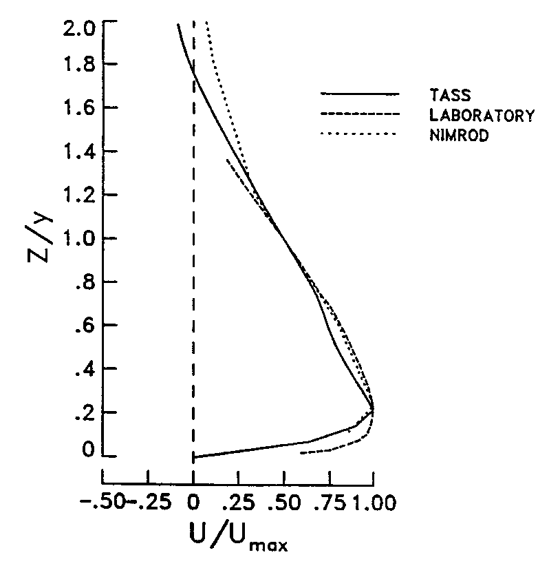
Figure 2 — Vertical Profile of Microburst Outflow (Non-dimensional)

Figure 2 shows dimensionless vertical profiles of horizontal velocity, u, for TASS data, laboratory data obtained by impingement of a jet on a flat plate, and data from NIMROD (Northern Illinois Meteorological Research on Downbursts) [ref. 13-21]. Specific points of interest are the maximum horizontal velocity (located 100-200 metres above the ground), below which is a decay region due to boundary layer effects, zero velocity at the stagnation point on the ground, and an exponential decay with altitude above the maximum velocity altitude. Vertical velocity profiles from TASS data are shown in Figure 3, also exhibiting a decay to zero at the stagnation point.

VERTICAL PROFILES OF VERTICAL VELOCITY FOR 30 JUN 82 CASE:
SENSITIVITY TO RADIUS OF PRECIPITATION SHAFT

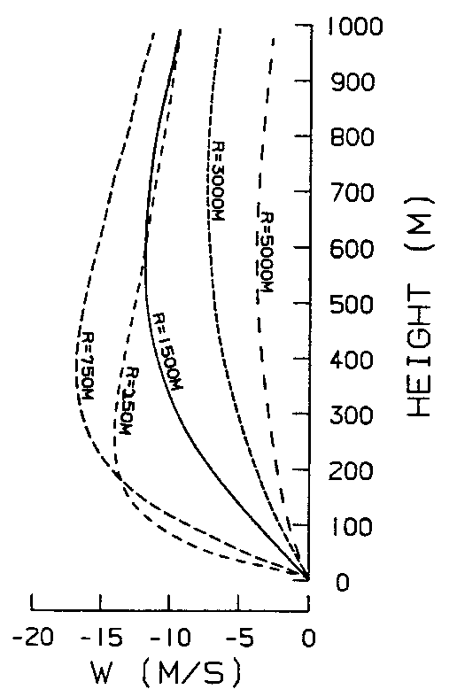
Figure 3 — Vertical Profile of Microburst Downflow

The radially varying characteristics desired for the horizontal wind were two peaks of equal magnitude and opposite direction located at a given radius, with a smooth, nearly linear transition between the two. Beyond the peaks, the velocity should show an exponential decay to zero. The vertical velocity was required to have a peak along the axis of symmetry (r = 0), and to decay exponentially as the radius increases.

A pair of shaping functions that gave velocity profiles matching the TASS data as required are given below.

The remaining solutions were found by integrating equations 4a and 4b, yielding:

Figures 4 and 5 show plots of these shaping functions.

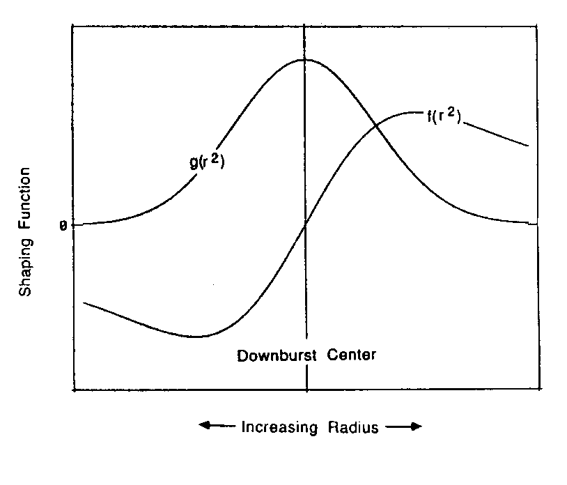
Figure 4 — Characteristic Variation of Horizontal Shaping Functions

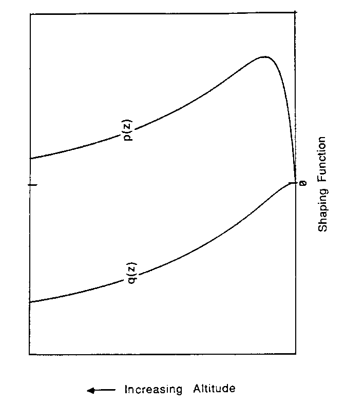
Figure 5 — Characteristic Variation of Vertical Shaping Functions

Combining the functions as in equation 3, the horizontal and vertical velocities are expressed as

(5)

(6)

By taking derivatives of equations 5 and 6 with respect to r and z, respectively, and substituting in equation 2, it can be shown that the velocity distributions satisfy continuity.

The parameters z* and ε were defined as characteristic scale lengths associated with ‘out of boundary layer’ and ‘in boundary layer’ behaviour, respectively. Analysis of TASS data indicated that z* = z_m2, the altitude at which the magnitude of the horizontal velocity is half the maximum value.

It was also noted that the ratio

To determine the location of the maximum horizontal velocity, the partial derivatives of u with respect to r and z were set equal to zero. The resulting equation for the r-derivative is

The resulting equation for the z-derivative is

Recalling that z_m/z* = 0.22, the values 1.1212 and 12.5 were obtained from iteration for the ratios r/R and z*/ε, respectively.

Using these values, the maximum horizontal velocity can be expressed as u_max = 0.2357 λ R. The maximum vertical wind is located at r = 0 and z = z_h, by definition, and is given by

A ratio of maximum outflow and downflow velocities can be formed

The Scaling factor, λ, was determined by using either of equations 5 or 6 for horizontal or vertical velocity, and setting it equal to the maximum velocity, u_max or w_max, respectively. Solving for λ results in:

The velocity equations were easily converted to rectangular coordinates, as shown in the Appendix. Partial derivatives with respect to x, y, and z were obtained by differentiating the velocity equations, and are also listed in this Appendix.

DISCUSSION AND RESULTS

Vertical and horizontal velocity profiles for u and w are shown in Figures 6 and 7.

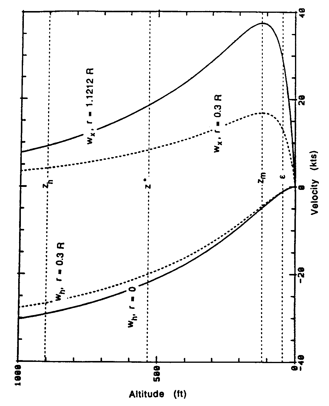
Figure 6 — Vertical Velocity Profiles for the Analytical Model

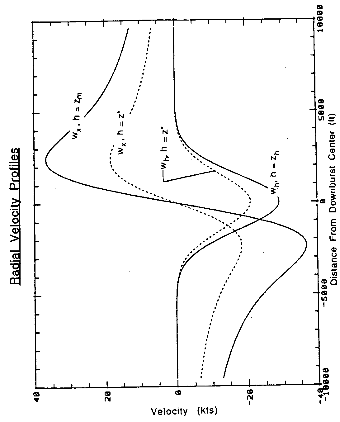
Figure 7 — Radial Velocity Profiles for the Analytical Model

Four profiles are shown for each component. The horizontal wind profiles in figure 6 were taken at the radios of peak outflow (r = 1.1212 R) and at about one-fourth that radius (r = 0.3 R), where the maximum outflow is approximately half the value at the peak outflow radius. The vertical wind profiles were taken at the radius of peak downflow (r = 0) and at r = 0.3 R. Horizontal wind and vertical wind profiles in figure 7 were taken at altitudes of h = z_m (maximum outflow), h = z* (half-maximum outflow), and h = z_h (depth of outflow).

This analytical model is compared with TASS, laboratory, and NIMROD data in figure 8. The figure shows that, when non-dimensionalised by the altitude of half-maximum outflow (z*) and by the maximum outflow (u = u_max), the analytical model agrees closely with the other data.

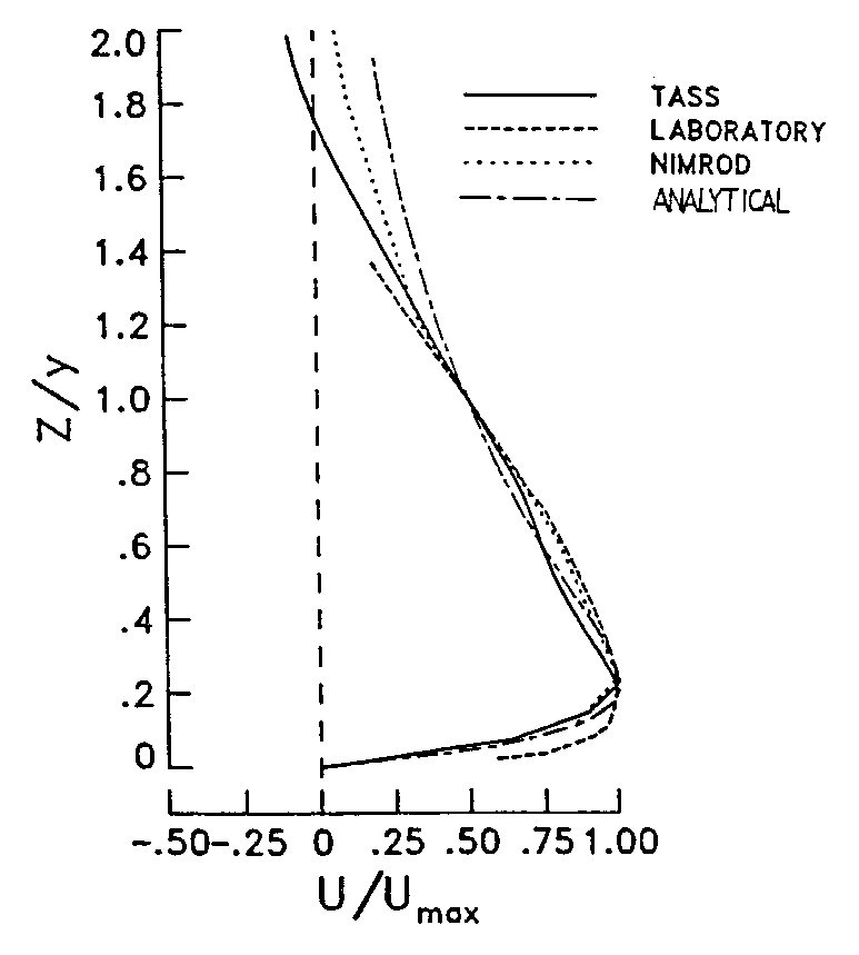
Figure 8 — Comparison of Wind Model Vertical Profiles

Different shears can be modelled by specifying four parameters, and the location of the downburst centre relative to the aeroplane flying through it. The four parameters are: 1) a characteristic horizontal dimension; 2) the maximum wind velocity; 3) the altitude of maximum outflow; and 4) the depth of outflow. The characteristic horizontal dimension specified is the radius of the downdraft column, noting that this is about 89 % of the radius of the peak outflow. The maximum wind velocity can be either horizontal or vertical.

CONCLUDING REMARKS

The analytic microburst model developed for use in real-time and batch simulation studies was shown to agree well with real-world measurements for the cases studied. The functions chosen for the model showed boundary-layer effects near the ground, as well as the peak and decay of outflow at increasing altitudes, and increasing downflow with altitude. The exponential increase and decay of the downflow and outflow (in the radial direction) are also characterised by the model. Equations for horizontal and vertical winds are simple and continuously differentiable, and partial derivatives in rectangular or cylindrical coordinates can be easily obtained by direct differentiation of the velocity equations. The governing equation for this system is the mass conservation law, and the analytic velocity functions developed here satisfied this condition. The model is sustained by a strong physical basis and yields high fidelity results, within the limitations of maintaining simplicity in the model, and variability of the microburst phenomenon. Parameterization of some of the characteristic dimensions allows flexibility in selecting the size and intensity of the microburst.

REFERENCES

1. Oseguera, M. and Bowles R. L.: A Simple, Analytic 3-Dimensional Downburst Model Based on Boundary Layer Stagnation Flow, Rosa, July 1988.

2. Bray, R. S.: Application of Data to Piloted Simulations. Wind Shear/Turbulence Inputs To Flight Simulation and Systems Certification, NASA CP-2474, 1987, pp. 97-115.

3. Hinton, D. A.: Aircraft Trajectory Guidance During Wind Shear Encounters. Master’s Thesis, George Washington University, January 1988.

4. Hinton, D.A.: Flight management strategies for escape from microburst encounters, NASA TR 4057, 29, pp. 1988.

5. Hinton, D.A.: Relative merits of reactive and forward-look detection for wind shear encounters during landing approach for various microburst escape strategies, NASA TM-4158, DOT/FAA/DS-89/35, 1990.

6. Proctor, F.H.: The Terminal Area Simulation System, Volume I: Theoretical Formulation, NASA Contractor Report 4046, April 1987.

7. Proctor, F. H.: Numerical simulations of an isolated microburst. Part I: Dynamics and structure, J. Atmos. Sci., 45, pp. 3137-3160, 1988.

8. Proctor, F.H.: The Terminal Area Simulation System, Volume II: Verification Cases. NASA Contractor Report 4047, April 1987.

9. Proctor, F. H., 1989: Numerical simulations of an isolated microburst. Part II: Sensitivity experiments, J. Atmos. Sci., 46, pp. 2143-2165.

10. Frost, W.: Modeling and Implementation of Wind Shear Data. Wind Shear/ Turbulence Inputs to Flight Simulation and Systems Verification, NASA CP-2474, 1987, pp. 49-66.

11. Proctor, F. H.: NASA Wind Shear Model -- Summary of Model Analysis. Airborne Wind Shear Detection and Warning Systems, NASA CP-10006, 1988, pp. 29-66.

12. Proctor, F. H., and Bowles, R. L.: Three-dimensional simulation of the Denver 11 July 1988 microburst-producing storm, Meteorol. and Atmos. Phys., 49, 1992, pp. 107-124.

13. Fujita, T. T.: Tornadoes and Downbursts in the Context of Generalized Planetary Scales. Journal of Atmospheric Sciences, vol. 38, no. 8, August 1981, pp. 1511-1534.

14. Oseguera, R. M.; Bowles, R. L.; and Robinson, P. A., 1992: Airborne In Situ Computation of the Wind Shear Hazard Index, AIAA Paper 92-0291, 1992.

15. Lewis M. S., Robinson P. A., Hinton D. A., Bowles R. L.: The relationship of an integral wind shear hazard to aircraft performance limitations, NASA TM-109080, 1994.

16. Arbuckle, P. D., Lewis M. S., Hinton D. A.: Airborne systems technology application to the windshear threat, 20th Congress of the International Council of the Aeronautical Sciences, ICAS Paper No. 96-5.7.1, pp. 1640-1650, 1996.

17. Airborne Windshear Detection and Warning Systems. First Combined Manufacturers’ and Technologists’ Conference, NASA CP-10006, DOT/FAA/PS-88/7, 1988.

18. Airborne Windshear Detection and Warning Systems, Second Combined Manufacturers’ and Technologists’ Conference, NASA CP-10050, 1990.

19. Airborne Windshear Detection and Warning Systems, Third Combined Manufacturers’ and Technologists’ Conference, NASA CP-10060, DOT/FAA/RD-91/2-1, 1991.

20. Airborne Windshear Detection and Warning Systems, Fourth Combined Manufacturers’ and Technologists’ Conference, NASA CP-10105, DOT/FAA/RD-92/19-1, 1992.

21. Airborne Windshear Detection and Warning Systems, Fifth and Final Combined Manufacturers’ and Technologists’ Conference, NASA CP-10139, DOT/FAA/RD-94/14-1, 1994.

[Amdt ETSO/16]